CHAPTER 16
Other Models of Territorial DivisionIn 1982 I applied for a National Science Foundation grant to extend the
We gathered state-level data on over 400 non-governmental units. A representative sample of these is shown in Table 16-1. Our initial purpose was simply to see whether businesses showed a distribution like We of course expected to find b = 2/3. A glance at the b-column of Table 16-1 shows that businesses very clearly did not fit the expected pattern. There are exceptions, to be discussed separately below, but the overwhelming majority of businesses show a slope closer to unity than to 2/3. Why? These results do not undo previous results. Governments studied previously still behave according to the size-density law. But it is disturbing to find here a whole set of units which behave differently. Do they need their own special theory, or can we generalize the earlier derivation (Chapter 10) to accommodate the new findings? Distance Exponent β: Clumps and Gaps Our problem was to reformulate the derivation so that the slope in Eq. 1 could vary from 2/3, taking a value near unity. The simplest way to achieve this was to add an exponent to S in the initial equation:
Minimizing T as before, we obtain
where k = (βwβ/hv)2/(β+2). Dividing by A results in with the logarithmic transformation
When β = 1, b = 2/3. As β → 0, b → 1, yielding the values obtained empirically for many of the businesses in Table 16-1. As service establishments, businesses differ from seats of government in at least one important way with regard to location criteria. Businesses do not locate in areas where there is little demand for their services. Where there is high demand, they compete with one another for the same market population. Businesses clump together in regions of high demand;. They also leave gaps where demand is low. In contrast, governments (e.g., county seats) must have access to every point within their jurisdiction. And everyone, no matter how low the local density of settlement, must have access to governmental services. Governments cannot permit gaps, nor can they clump together to form overlapping service areas. The significance of the areal factor is reflected in the value of β, the exponent on distance in Eq. 2. It has been well established that, at the micro level (within a city), distance from potential clients plays a role in business location decisions. At the macro level (inter-state comparisons) local distance is irrelevant. The diminished effect of distance at this level will be reflected in a value of β tending toward zero. Local governments, which must serve both a population and an area, should be expected generally to show values of β tending toward unity: every square mile counts. Adding an exponent to distance sheds light on a persistent finding in previous research, namely, the tendency for governmental density slopes to erode from 2/3 toward zero. A slope less than 2/3, with β > 1, suggests that distance is playing even more of a role in location patterns than physical reality or the theory of time minimization would lead us to expect. It is the reverse of the pattern observed for businesses: any redistribution of population is more-or-less actively ignored as governments remain fixed in place. Gaps in governmental service appear in heavily populated areas, a tendency to clump in lightly settled ones (note, for example, the relatively few county seats in Southern California as opposed to the number in the Gold Rush region of the Sierras). The inefficiency of such an arrangement must, of course, be viewed in the wider context of overall time-efficiency. It is expensive, in many senses, to overcome inertia and re-organize entire systems of local government. In the meantime, β > 1 describes the condition. Population Exponent α: Economies of Scale Research has concentrated on Eq. 1 relating the density of establishments to the density of population. But, as we saw above, Eq. 3 can also be tested directly, from the logarithmic transformation
It is evident algebraically that the two regression coefficients in this equation must sum to unity. Yet the coefficients f = 2/(β+2) and g = β/(β+2), as shown in Table 16-1, do not in general sum to unity. Many come close, initially suggesting simple rounding errors, but some (e.g., #24, bookstores) total as low as .76. Another (#3, bicycle shops) totals 1.36. Such departures from unity are not due to rounding. Something is wrong with Eq. 6. We only have two independent variables [2], one of which has already received an exponent. What would happen if we add an exponent to the other independent variable, P?
This leads by the same procedure as before to
with coefficients which sum to unity only when α = 1. If β were equal to zero, the antilog form of Eq. 8 would be N = kPα. Thus, α describes the relation between N and P independent of distance and area. The complete absence of geographic constraints may seem far-fetched (a society of angels or Platonic souls, "beam me up" forms of space travel), but there are some real-world instances where geographic constraints are simply ignored. Seats in Congress for example, are apportioned on a strictly percapita basis. This method of distributing congressional seats makes β = 0 automatically. As a consequence, congressional districts vary greatly in size (1 member of Congress for the entire state of Alaska, 2 for the city of San Francisco). In this special case α = 1: The population served by each member is a constant (1/k), and congressional delegations, by constitutional intent, increase as a simple linear function of population growth.
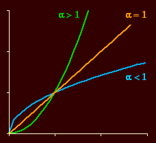
When α < 1, as for many services in Table 16-1, N grows at a decelerating rate with respect to P. Increasing values of P lead to increasing values of N, but at a slower rate. Existing establishments absorb much of the increased demand. Conversely, α > 1 describes an accelerating rate of increase in N with respect to P. Establishments are sparse where P is small, but increase rapidly for large P values. Establishments in areas of high population density serve a smaller clientele than do those in sparsely settled areas. These conditions can be illustrated by the way in which different religions establish churches for their members. If a denomination routinely divides one congregation into two when the membership increases beyond a certain point, congregations would tend to be of constant size and as a result α = 1. This is nearly the case for Baptist churches, #44 in Table 16-1. Denominations which respond to increased membership by adding more hours of service at the same locations would produce α < 1, as in Catholic churches, #45. The denominations which operate through small "store front" churches in large cities would illustrate α > 1; unfortunately there are no national data for such denominations, so we have no empirical example here. Measurement of α and β While the introduction of α and β permits theory to be general enough to reflect empirical fact, it also introduces a measurement problem. In Eq. 5 the independent variable was simply P/A; we now have Unless α = 1, its effects will be confounded with those of β in determining the slope b. Clearly, α and β must be measurable if Eq. 9 is to be anything other than a useless formalism. The solution to the measurement problem can be obtained from Eq. 8. The measurement of β derives algebraically from the formula for g, the coefficient on log A. Since it follows that
This result can be substituted in the formula for the coefficient f on log P Characteristics of Particular Services Table 16-1 entries #1-14 show two sets of values for various businesses. Those suffixed with "p" show statistics describing the density of service establishments in relation to the density of total state populations. In previous studies of county governments, it was found that the slope b came closer to the expected 2/3 value if the independent variable referred to the density of the rural population only, the principal market for such governmental services. I could not obtain data regarding the market populations served by the businesses studied here. Figures were available, however, on the total receipts for each kind of business. It seemed reasonable to assume that, for the purpose of state-by-state comparisons, the volume of receipts could stand as a proxy for the relative size of state market populations. All non-suffixed entries in Table 16-1 were computed with receipt density (or, if you will, the density of the receipt-estimated market populations) as the independent variable.
In general, results for market populations are closer to theoretical
expectations than those for total state populations. Both sets of
findings, however, support the contention of a slope nearer unity than
2/3. The lowest b-value is .73 (#7, drive-in theaters, p); the value for
market population (#8) is b = .87; and, adjusted[3] bα = .96.
#7's f and g coefficients look like governmental values expected from
Eq. 15-1, (f = .68, g = .22). When the market population is used, #8,
they look more like what we expect for a business (f = .75; g = .04).
β also changes, from .57 to .09, as we would expect. This dramatic
reduction in the value of β, as we shift from total to market
populations, is evident throughout #1-14. Gas stations
(#15-17) provide a slightly more refined illustration of the
tendency for β to approach zero as we approach the market
population more closely. For the total state population, β = .24;
for the population of licensed drivers, β = .11; for the market
population β = .06. Several businesses have a very unusual
market distribution vis-à-vis the distribution of the general
population. The slope for farm supply stores (#18), estimated from the
total state population, looks close to 2/3 (b = .62), but this is
obtained from a combination of really extraordinary values of α and
β (α = 1.43; β = 1.84). The receipt-estimated market
population produces results which make farm supply stores appear at
least statistically like other business (b = .88; α = .95; β =
.20). Mobile home dealerships (#20) show a similar initial slope of
almost exactly 2/3, but it is produced by other α and β values
(α = .99; β = 1.02). This looks initially like the pattern
found for seats of government, but when market populations are used the
pattern is typical of those obtained for other businesses (b = .96;
α = .93; β = .02).
Entries #22-43 show results for the market
populations of a number of other businesses. In general, b is near
unity. The two possible exceptions are #29 and #34 (electrical supplies,
plumbing and heating), with b = .76 in each case. Both have unusually
high β and low α values. The α-adjusted slopes are closer
to expectation (.91 and .84). In all cases the α-adjustment has the
effect of increasing r2, though the increase on values which are
already quite high may not be noticeable due to number of decimal places
shown. It may also be noted that The distribution of the two kinds of churches has already been mentioned above in connection with the interpretation of α. The diocesan structure of the Catholic church, as opposed to the congregational structure of the Baptist, would lead us to expect higher values for β and g, the two distance/area coefficients; they are, in fact, about twice as high for Catholic as for Baptist churches. The f coefficient for Catholic churches (.64) is almost exactly the theoretical 2/3 value we would expect for governments; since g (.21) falls short of 1/3 and the α-adjusted b is .79, it would appear that the distribution of Catholic churches lies somewhere between the purely governmental and the strictly market-oriented pattern. #46 and 47 show interesting patterns distinguishing them from other service establishments. In the tradition of biological ecology Park [4] long ago noted the tendency of businesses to be distributed (as they are in the data reported here) according to the distribution of their "food supply," namely, receipts. What is interesting is that he was specifically referring to the geographic distribution of newspapers, in relation to subscribers, advertisers, and other sources of income. Whatever may have been the case in his day, newspapers (#46) now appear to be distributed more like governments than businesses: b = .58. Nearly every locality has one newspaper (no gaps) and — as major urban newspapers are forced to either consolidate or go out of business — even very large population centers support only a few (no clumps). The result is that newspapers approach the governmental pattern (b = .69, bα = .77; f = .62, g = .23). Hospitals come even closer to the governmental pattern (b and bα = .68; f = .68, g = .32; α and β are nearly unity), and here the reference is not to receipts but to the distribution of the general population, i.e., the potential market for their services. That α = .99 means that, in the absence of distance factors, there is a linear relation between the population served and the number of hospitals. That β = .92 means that all areas are served (no gaps) and that, even in large centers, hospitals don't appear to compete with one another in the sense that most businesses do. Whether through their own location decisions or the fact that they are heavily regulated in the public interest, hospitals demonstrate an almost perfect service-oriented spatial distribution. County seats (#48-50) appear to have shown a similar distribution with regard to the rural population in 1920. By 1970 this condition had clearly changed, and in the direction opposite to the pattern established in business. Even with respect to the rural population β had changed from 1.14 to 1.84; with respect to the total population it becomes 2.33. It is obvious that there is a rural bias in the distribution of the nation's 3,000-plus county seats; and, even among the rural population, there is a bias in favor of providing seats to lightly settled areas. Non-governmental service establishments appear to be constrained to redistribute themselves. Empirically, they seem to respond to changes in the distribution of opportunities to make money (businesses) or to provide services (hospitals) or both (newspapers). Governments appear to be above such constraints. Once established, their distribution is very resistant to change. If county governments were subject to the time-efficiency requirements of hospitals, many of them would be out of business, consolidated into oblivion as were many rural school districts with the advent of the school bus. Apparently social inertia — together with the power of governments to tax, to legislate and to judge — confers a special respite from the constraint of time minimization, at least in the short run historically. If county seats are "hypo-governmental" (b < 2/3), physicians (#51) appear to be "hyper-business" (b > 1), more unevenly distributed than the distribution of their potential market would suggest. β < 0 suggests an impossibility in strictly physical terms (going a shorter distance takes more time?). Perhaps the interpretation here should be that through professional organization physicians have freed themselves from normal market constraints, enabling them to concentrate in much greater numbers in high density regions. The flip side of this arrangement is that it also results in extreme gaps in service to low density areas, with even less service provided than the market in such areas would call for. Service Delivery Methods Behind the dry statistic β lies a fundamental contradiction in the ways in which services can be provided to a distributed population. This difference was brought home to me in another case, namely, the distribution of gas stations. Oddly, the earliest of the size-density derivations (Mycielski and Trzeciakowski, Chapter 8) dealt with providing a cost-efficient distribution of gasoline service stations; they suggest that their model was employed for this purpose by the planning officials in Poland (at that time a nominally Marxist state under Soviet hegemony). Their derivation leads to an expected b = 2/3 or, in terms of the new derivation, β = 1. When I first began this research I did not find the application unusual since all theory led to the same expectation. Yet the data on the distribution of gas stations in the United States showed b = .96 and β = .04 (this is for the market population, but that is the population presumed in the Mycielski and Trzeciakowski derivation). I believe the value of β reflects a real difference in general strategies of service delivery. When β = 0, provision of services takes place in response to market conditions, with competition resulting in clumps and gaps in service. If β = 1, service takes place through a set of mutually exclusive and space-exhaustive service areas, the pattern I have associated with ideal governments. The advantages and disadvantages of the two strategies are apparent: When β = 0 there is competition for receipts, resulting in some gaps in service but also resulting in a choice among service providers, at least in high density areas. In contrast, when β = 1 there are no gaps in service. But there is also no competition, no choice among service providers. Each market population is provided with one, but only one, gas station. Just as businesses run the risk of being hypercompetitive (like physicians in this study), such government-businesses run the risk of becoming unresponsive to changes in market conditions (like the county seats in this study).
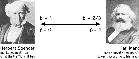
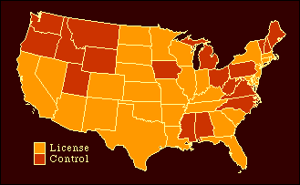
β seems to identify two polar types, from the Spencerian ideal of pure capitalism where β = 0 (what the traffic will bear) to the Marxian ideal of pure communism where β = 1 (to each according to his needs), with pathological extremes beyond either limit. The Distribution of Liquor Stores In the Spring of 1986 I found a unique opportunity to test the government vs. business view of spatial distribution. With the help of Hugh Phillips, a Sociology undergraduate, I studied the distribution of liquor stores. These were ideal for my purpose since liquor stores deliver essentially the same specialized product nationwide, but they do so under two completely different institutional arrangements. In 30 of the 48 contiguous states liquor stores are established as licensed businesses while in the remaining 18 they are governmental agencies.[5] The obvious question is: Will "license" states show a pattern typical of private businesses (β → 0); will "control" states show the governmental pattern (β → 1)?
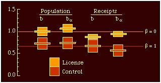
Table 16-2 shows statistics similar to those presented earlier in this chapter, except that the slopes are shown with their 95-percent confidence intervals.[6] These make possible the graphic presentation in Fig. 16-3 which clearly shows a difference in license and control states with regard to the geographic distribution of liquor stores.
The advantages and disadvantages of each type of spatial distribution were mentioned above: When β = 1, b = 2/3, all areas are served (space-exhaustive, no gaps), but each service area is served by only one center (mutually exclusive, no choice among service providers). When β = 0 so b = 1, there is clumping of service centers in high density areas and hence a choice among service providers. But there are also gaps in service where density is low; there are as many, but only as many, locations as the traffic will bear. The f-coefficients show fairly similar values across the board, indicating the strong dependence of liquor stores on the distribution of population regardless of license or control status. The two systems differ notably, however, with respect to the g-coefficients. On the assumption of a strictly space-exhaustive, mutually exclusive distribution β = 1 so g = β/(β+2) = 1/3. The theoretical value is approximated for the control states (.26 for total population, .44 for receipt-estimated population), but not at all for the license states (g = -.07 and .06). Area, hence distance, appears to be an important factor in determining the distribution of control liquor stores and of very little significance in determining the distribution of license liquor stores. There are also interesting differences between license and control states with respect to the α-exponent. In both population and receipt analyses, α is higher for control states than it is for license states. As already noted, if α were lower than unity it would mean that economies of scale resulted in larger liquor stores in densely settled areas (a "supermarket" pattern). If α were greater than unity, there would be more and more little stores as population increases (the "ma-and-pa market" pattern). Using the population figures, both systems seem to follow the supermarket pattern with the license states doing so much more markedly. If receipts provide a better estimate of actual use, however, there is a clear difference in the two, with control stores following the ma-and-pa pattern. This could be interpreted to mean that the development of service locations under market (business) pressure produces scale- economies. Such economies don't seem to emerge when development takes place under governmental control, where each additional store manager protects his or her own small turf free of competitive constraints.
NOTES: [1] The grant was SES-8215441. The results were published as G. Edward Stephan, "The Distribution of Service Establishments", Journal of Regional Science, 28:29-40, 1988. [2] T "looks" dependent while N "looks" independent, given their locations in these equations. But we are assuming T is fixed and N is to be determined. The only independent variables are thus S and P. [3] the last two columns of Table 16-1show the slope and coefficient of determination, recomputed after raising P-values to the power α. [4] Robert E. Park, "The City: Suggestions for the Investigation of Human Behavior in an Urban Environment", American Journal of Sociology, 20:577-612, 1919. [5] The classification of states as "license" and "control" came from the 1981 Annual Report of the Distilled Spirits Council. The control states are Alabama, Idaho, Iowa, Maine, Michigan, Mississippi, Montana, New Hampshire, North Carolina, Ohio, Oregon, Pennsylvania, Utah, Vermont, Virginia, Washington, West Virginia and Wyoming. [6] Confidence intervals for regression. These will be covered in the methodological appendix( [7] The number of liquor stores and their annual receipts, by state, came from the 1977 Census of Retail Trade. |


