|
CHAPTER 10
Random Numbers and a New Derivation
The size-density hypothesis led to the development of time- minimization theory, from which five other laws can be derived. But the size-density relation had never been tested for the topic where it was, in a sense, born: counties of the United States. The absence of county area data prior to 1930 made statistical tests impossible. Toward the end of Fall term, 1978, an undergraduate majoring in Visual Communications, Doug McMullin, asked me to participate in his video-tape senior project (he had taken an introductory course from me several years earlier and needed some demographic information for the project). Doug entered the Sociology M.A. program the following June, and we worked on several projects together, one reported here and another in Chapter 12. A Density-Density Equation According to the size-density law, if a county lies in a region of density D its expected area would be A more traditional meaning of "expectation", in statistics, is the average where A is the area of the region and N is the number of counties in it. If the region's density D = P/A, we have
or, inverting the left side, which may be thought of as a relationship between the two densities: So we formulate the hypothesis and test it with region-level P, A and N data. The units of analysis for our study were all states and territories for which historical data were available.[1] In several cases we used units for which data were available even when they did not have state or territorial status, e.g., Maine (which was part of Massachusetts until 1820) and West Virginia (part of Virginia until 1863). Previous research suggested that the independent variable should be made as specific as possible. We were able, with the data available, to calculate rural densities as well as total densities. We did so since the theory did not address urban clumps within territorial divisions; also, the 2/3 line developed for the world no doubt reflected primarily rural populations. The initial results of our analysis are shown in Table 10-1 and Figs. 10-1 to 10-3.
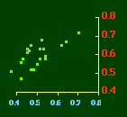
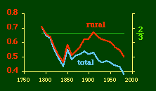
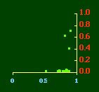
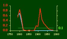
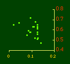
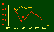
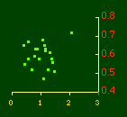
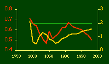
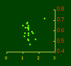
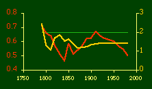
In the early years of this nation the population was almost entirely rural, therefore both independent variables produce virtually the same results. Increasingly, however, rural density diverges from total population density, and it shows results more in conformity with theory, as we thought it might. The left side of Fig. 10-1 shows a scatter diagram relating rural density values (Y-axis) to total density values (X-axis). As Fig. 10-1 shows, the slope for rural density fits the theoretical 2/3 value at the birth of the nation — after 200 years of occupancy and just prior to westward expansion. With expansion it declines, presumably because population spread faster than county seats did. It then rises briefly in 1850, due I believe to the addition of Texas and California: each had long-established systems of local government under Mexican rule, and these were simply converted to counties on admission of the states to the Union. After that the slope generally rises again toward the theoretical 2/3 value With the closing of the frontier and the introduction of the automobile, it drifts toward zero again since subsequent population shifts no longer bring about the creation of new counties. Figs. 10-2 and 10-3 strengthen these conclusions.
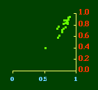
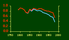
Obviously, both total and rural density correlated fairly highly with each other (left side of Fig. 2) and throughout the period, though each has been declining since the first part of the 20th century.
Here there is a dramatic difference between rural and total population density. The total density departs rapidly and permanently from the 2/3 value. Its high coefficient of determination and increasing number of cases guarantee that it must fail as the slope departs from 2/3. Rural density, however, falls away and then clearly returns to 2/3 (probabilities well above 0.10) with the closure of the frontier. Since then, due to the arrival of the automobile, the slope has been falling away toward zero, so the probability associated with 2/3 has likewise been on the decline. The Result of Random Numbers? But what about randomness as the source of the 2/3 slope? Recall from Chapter 8 that the -2/3 size-density slope could be obtained from random numbers. What about the positive 2/3 slope of Eq. 2? Beginning with the slope formula as before
and substituting, we arrive at the ungainly
Ungainly or not, it produces the anticipated result: random numbers for P and N, together with multiplied pairs of random numbers for A as before, produce Substituting these in the "reduced" version of Eq. 3 produces
So is all this to be written off as the result of statistical computations on random numbers? Table 10-2 shows our computations for the relevant variances, covariances and ratios needed to test this idea.
Table 10-2 shows that none of the covariances stabilize at the value of zero expected under the random numbers hypothesis. Nor do the ratios hover around the expected value of two. Let us look at each of these expectations in turn, in relation to changes in the slope relating center-density to rural-density.
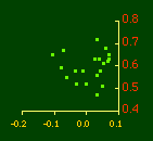
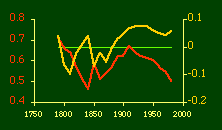
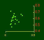
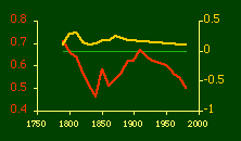
The left side of Fig 10-4 shows that the covariance(P,A) is unrelated to the value of b. If we look at their values over time (right side) this becomes very clear. The expected values — b = 2/3 & cov(P,A) = 0 — are shown by the horizontal line. Both are near these values in 1790. During the 19th century they approach and depart from these values in opposite directions. In 1910, when the slope has returned to its time-minimizing value, the value of cov(P,A) is as far above its random-numbers value as it ever gets. As it returns toward zero, the slope departs from 2/3. Figs 10-5 and 10-6 show that the covariances (A,N) and (P,N) are similarly unrelated to the slope, as raw values (left sides), or over time (right sides). This shows most clearly after 1900 — as the slope decays cov(A,N) remains constant (no new states, very few new counties) and cov(P,N) approaches zero.
The same thing seems true of the variance ratios shown in Figs. 10-7 and 10-8. Each should equal 2, according to the random number argument. The only point at which they approach this value is in 1790. After that they don't behave as we would expect in connection with the 2/3 slope. State values for A and N are virtually unchanged through most of this century; the other ratio drifts toward a value of 2 while the density-density slope drifts toward zero.
I was on sabbatical leave in Greece, California and Washington, D.C. during 1980/1, but stayed in contact with Doug who was house-sitting for us and working on his M.A. thesis (see Chapter 12). We published the results reported here in 1981.[3] A New Derivation from Time-Minimization Sometime in 1981 I realized that the "density-density" equation, Eq. 2, could be derived directly from considerations of time minimization, without going through the size-density derivation as an intermediary step. The result is a set of four equations, one of which is the original size-density equation. We begin as before with the assumption that social structures evolve in such a way as to minimize the time expended in their operation. We also retain the notion of maintenance time and interaction time. The only difference now is that we no longer focus on the size of a single county. Rather, we ask How many counties should a region have, given its population and area? Maintenance time will refer to the total time cost required to provide the state with N counties. With h as the average cost per county, total Interaction between residences and county seats will require travel. The average distance S is traversed at the average velocity v. The P individuals making roundtrips will expend an Both these statements are true by definition: They state only that an amount may be expressed as an average (h or S/v) times the number of cases (N or P) . The time expended in the operation of the N counties is given by the sum In the earlier derivation we expressed the average distance as function of county area. This was a consequence of dimensional analysis. Here again we express average distance as a function of the square root of area, but it is now the average area for the set of N counties. The average area will be the total region's area A divided by N. Thus, with w as the constant of proportionality, We re-write the equation as differentiate with respect to N, set equal to zero and solve for N
where k = (w/hv)2/3. The number of counties which will minimize time is thus given as a function of the region's population and area. Algebraic manipulation produces four more equations. Division of Eq. 10 by A produces Division of Eq. 10 by P produces Inversion of the left side of Eq. 11 results in Inversion of the left side of Eq. 12 results in Eq. 11 is identical to Eq. 2 derived from expectation algebra. Eq. 12 is the parallel to Eq. 11.; the latter gives the density of county seats, the "center density" (C = N/A), while the former gives county seats per capita, the rate (R = N/P). Eq. 13 is the original size-density equation, except here the term on the left refers to the average county size in a region rather than the size of a given county. Eq. 14 is a parallel to Eq. 13; it gives the average population per county. (I use lower case "a" and "p" to distinguish these from regional areas and populations.) The relation among the four equations is shown in Table 10-3 (with D=P/A, C=N/A, R=N/P, a=A/N and p=P/N):
The algebra is tedious (you can see it here), but it can be established that these four equations are statistically equivalent. That is, testing one of them is, in effect, to test all. It would thus appear to be a matter of convenience (which kind of data are available) — whatever equation is tested, the other results can be calculated algebraically. None of this was easy to get published.[4] Appendix — Exact Probabilities It is traditional in the social sciences to report findings at various significance levels, e.g., p < .01 or p < .05, just as I have done in earlier chapters. I switched, with the work reported in this chapter, to reporting exact probabilities. The change was partly due to the fact that it became technically possible for me to do so around this time (see below). I also did it because I agree with Lehmann's argument: [5] It is ... good practice to determine not only whether the hypothesis is accepted or rejected at the given significance level, but also to determine the smallest significance level ... at which the hypothesis would be rejected for the given observation. This number gives an idea of how strongly the data contradict (or support) the hypothesis, and enables others to reach a verdict based on the significance level of their choice.Until the advent of modern computers we had to rely on tables of the t- distribution to report significance levels. Around the time of the research reported here, programmable calculators and personal computers made it easy to evaluate the integral describing the distribution. You can see the BASIC program I used here
NOTES:
[1] The source for historical population and area data was Bureau of the Census, Historical Statistics of the United States, Colonial Times to 1970. Series A:195 (Population) and A:211-61, Washington, D.C., 1975. The number of counties per state was from Table 2-1. [2] The caption symbols refer to logged values, e.g., D stands for log D. [3] G. Edward Stephan and Douglas R. McMullin. "The Historical Distribution of County Seats in the United States: a Review, Critique and Test of Time-Minimization Theory", American Sociological Review, 46:907-17, (1981). [4] The new derivation and the skeleton the argument of Eqs. 19-32 was published as G. Edward Stephan, "Territorial Division", Social Forces, 63:145-158, 1984. As in most Sociology journals, the typesetting made the equations virtually unreadable. [5] E. L. Lehmann, Testing Statistical Hypotheses, :61-2, New York: Wiley, 1959. | |||||||||||||||||||||||||||||||||||||||||||||||||||||||||||||||||||||||||||||||||||||||||||||||||||||||||||||||||||||||||||||||||||||||||||||||||||||||||||||


