CHAPTER 9
Time-Minimization and Other Laws
A theory ought to do more than account for the observation which prompted its formulation. The hope is that a theory which accounts for one general class of events might account for another. The classic case is Newtonian physics, where the law of universal gravitation accounts for such diverse phenomena as falling objects on the Earth's surface, the motion of the Moon around the Earth, the rise and fall of tides, the behavior of ballistic projectiles, the movement of the planets around the Sun and the trajectories of comets. But this is simply the best-known instance of a standard pattern. Consider the development and generalization of germ theory.[1] In 1847 Ignaz Semmelweiss reduced the number of cases of childbed fever by having surgeons wash their hands before deliveries. In 1865 Joseph Lister reduced infections by washing patients' wounds with carbolic acid during surgery. William Budd stopped a cholera epidemic in 1866 by controlling Bristol's water supply. Louis Pasteur demonstrated in 1881 that sheep injected with weakened anthrax bacteria did not develop the disease. A year before Charles Laveran had discovered a protozoan, not a bacterium, in the blood of a soldier suffering from malaria. The germ theory of disease was so successful [2] that organisms too small to be seen or trapped in filters (viruses) were postulated to explain communicable diseases like measles. The theory is so entrenched that even diseases which are non-communicable (cancer, diabetes, multiple sclerosis) have been thought to be caused by a "germ". This chapter reports several attempts to extend the scope of time-minimization theory, generalizing it to empirical findings other than the size-density relation. I realize that in some of these efforts I appear to be walking very far out on very thin ice, both empirically and logically. Only further research, of course, can determine whether the effort was worthwhile. Area of Cities Within a month of developing the size-density derivation from time-minimization I started working on another involving the area and population of cities. Stewart and Warntz[3] had reported a relationship involving a three-fourths slope where A is area, P is population and K is the intercept. The relationship is shown for cities in England and Wales in 1951 (Fig. 9-1). They also showed a 3/4 slope for cities in the United States in 1940.
Incidentally, I first became aware of this relationship in an article by Ogburn and Duncan,[4] where the equation appeared as This literally says that A = .2P or area equals one-fifth the population. Their next sentence said this implied a 5.6-fold increase in area for every 10-fold increase in population which is not true. It turns out that in the original article the equation was given as If someone wrote 3/4 as .75, then overlooked the period, then reversed the last two digits of the denominator in the constant, that would have produced the misprinted form of Eq. 1. To continue, I knew I couldn't just apply the earlier derivation directly: first, because the relation depended on population rather than density; second, because the slope here is positive and the size-density slope was negative; and third, because cities don't develop through a process of division — they grow around points in space, and their boundaries may or may not be contiguous. A city is a "central place" — everyone who interacts with a city spends travel time doing so. As before, we can represent this as the average distance divided by the average velocity of the means of transportation. People in cities compete with one another for a place to live. The more people per unit area (the greater the density), the greater the competition. We can express this time expenditure (e.g., rent from income from labor time) as As before, we have a centripetal force (interaction) tending to draw people together, contradicted by a centrifugal force (residence) tending to push people further apart. And, as before, we sum the interaction and residence times By dimensional analysis substitute S = wA1/2 to obtain and re-write Finding the minimum and solving for A This is obviously not the same as Eq. 1, but we are not finished. We have only looked at the city as a place to live. Cities are also centers of commerce and trade. Just as residents must face competition for living space, described by density, merchants must face competition for a share of the market. We can represent this competition with the "market potential" [5] (dimension: people per mile) which we can put, with the appropriate substitution, in place of competition for space in Eq. 3
proceeding as before. The two functions of cities — as places to live and as places to trade — thus produce two different expectations regarding city area. Of course these are purely imaginary types of cities. Real cities perform both functions. We need to draw back from these extremes (a slope of 2/3 for the residential city, unity for the market city). Should we "split the difference" half-way, at 5/6? We could, but there is another possibility based on the kind of data available. The census distinguishes cities and urbanized areas. Cities are legally defined, incorporated areas. They may include much unoccupied land; they may exclude much territory demographically and economically bound to themselves. To tap the urban "reality" (independent of the legal definition) the census bureau designates "urbanized areas" regardless of legal status. I decided to "split the difference" by making hypotheses out of the two central relations, Eqs. 7 and 8: Lucky Tedrow and I analyzed data from three censuses (1950, 1960, 1970 — the three at the time which provided data for urbanized areas) to test these hypotheses. The results are shown in Table 9-1.
The observed slopes did not differ significantly from expected (p > .05). Each did differ significantly from the slope expected for the other type (i.e., city vs. urbanized area, p < .0001). We wrote up these results in the Fall of 1975 and they were published[6] shortly afterward. Given the delay in getting the size-density derivation published, this was the first opportunity to present the theory of time-minimization in print.
Lucky later found an earlier paper[7] we
could have cited. They reported a slope of -0.196 for the log of "land
provision" (the inverse of density) against log of population for a set
of cities in England and Wales about 1960. If we take the inverse,
density, at D ∝
P.196
and substitute D = P/A, we get the result A ∝ P.804, a result which agrees with our findings, but not
the earlier figure from Stewart and Warntz.
One further study involved extending the range down to much smaller
cities. The British cities in the Stewart and Warntz study were 50,000
population or more. Their U.S. cities were 25,000 or more. In 1940
cities of this size or greater represented only 12 percent of all urban
places (2,500 or more). The cities in the study I did with Tedrow
represented less than 6 percent of urban places. In the Fall of 1978
I completed study of smaller cities with another undergraduate, Rob Moe.
The 1970 census listed 6,435 places of 2,500 or more population. One
difficulty with this list was that it included "places" which were not
really cities (or towns or villages), places which were actually minor
civil divisions (some, but not all, of the townships in New England,
some boroughs in Pennsylvania and New Jersey). We eliminated from the
study any place with a population density of less than 1,000 per square
mile (most of the township divisions we could identify had densities
lower than this). The slope b = .806 for our ten-percent random sample
(N = 572) did not differ significantly from the theoretical 7/9 value (p
> .20), but it did differ significantly from 3/4 value reported by
Stewart and Warntz. Most writers on the topic of city size have
pointed out that New York City is too small for its population (hemmed
in) and that Los Angeles is too large (spread out). This study would
support such claims: our national regression line would give New York a
size of 767 squares miles (it has but 300), and Los Angeles would be 338
rather than its 464 square miles. Comparing large and small cities using
our regression line, we found for the largest city in our state
(Seattle, WA) an expected value of 88 square miles (the actual value is
83). A very small town just north of Western Washington University
(Lynden) produced an expected value of 1.3 versus its observed 1.4
square miles.
Population Distribution Within Cities
Virtually every introductory Sociology text presents Burgess'
"Concentric Zone" theory of city structure.[8] The original model is shown in Fig. 9-2,
as originally labeled, reflecting turn-of-the-century land uses and
transportation technologies ("workingmen" walked to work, "middle class"
road the street car, "commuters" road the train).
One can argue the merits of the concentric or other zonal patterns in describing the real world.[9] My interest is in deriving it from time-minimization theory. The greater the distance from the central business district, the greater the travel time, given an average velocity for a given transportation technology. Under the assumption of time-minimization, therefore, distance is a centripetal force, tending to push the population inward.
In general, the greater the demand the higher the price. If everyone wants a central location to minimize travel time, it will tend to make central locations more costly than outlying ones. Since it takes time to accumulate money, this means that the centripetal force (travel time) creates its own centrifugal force (time expenditures to meet land costs).
The center marks the point of least aggregate travel time. Since businesses are interested in drawing the aggregate to themselves, they pay the higher cost of such central locations. Those with time to spare (bankers, executives) occupy the distant locations out of town. Most people will be located where the joint effect of these competing time- costs is minimized, as shown in Fig. 9-2d.
The early interest in concentric zones tended to focus on the "zone in transition", the area about to change from high density residential use to commercial use with growth in the central business district. It was here that "commercialized vice" (gambling, prostitution, speakeasies) was to be found. As businesses, such activities would tend to seek a central location. But the central location contains expensive property, and that tends to be watched by police. Since these businesses were illegal, they took the next best location, in the zone in transition, often up several floors from the street. These areas were not worth anyone's time to police, so the businesses were relatively safe. The concentric zone model is almost always followed in textbooks with more recent modifications, notably Hoyt's "Sector Model"[10] and the Harris and Ullman "Multiple Nuclei Model".[11] Neither of these violates time-minimization theory. For example, as downtowns became congested (with the growth of office buildings and the use of automobiles), it actually took more time to travel downtown (and park) than it did to go out of town, to a suburban shopping center. Land there was also cheap enough to provide parking places. The "multiple nuclei" pattern is a time-minimizing pattern. Gravity Model An equation[12] describing interaction between places (originally called the "gravity model" because of its formal similarity to Newton's law, also called the "interactance hypothesis") is where I is the amount of interaction (e.g., migration, trade, travel, communication) between places i and j; P is the population at i and j, and D is the distance between i and j. The three factors on the right side were often computed and plotted as a joint independent variable; k was then the slope of a regression line through the thus-generated "bi-variate" data points. Later models[13] add estimation of exponents for each of the three independent variables, but that is beyond our concern here. The model is easily derivable from time-minimization theory. Assume the probability of going from place i and place j is inversely proportional to the time its takes to go from one to the other. Assume also that the probability of interacting with place j is inversely proportional to the time it will take at j to obtain whatever is unobtainable at i. We can combine these two assumptions in the expression The first factor is a direct function of distance and an inverse function of velocity In general, the larger a place is, the more likely we are to be able to find the variety and quantity of goods and services we might need[14] (unless what we need is the absence of people[15]). Thus, We can substitute these in Eq. 9 We have only to multiply the probability of interacting from i to j by the number of people exposed to this probability, the population at i, to obtain the number of interactions from i to j The constant of proportionality k strongly reflects the velocity of transportation technology, as early recognized by the "father" of migration research.[16] An Aside: Application of the Gravity Model In the Winter of 1974 one of our graduate students, John Ullis, informed me that he had to drop out of the program (his father had died suddenly and John was needed in the family business). I suggested that since he had already done the course work he look for a "quickie" thesis topic and take the degree. The topic he settled on was testing the gravity model, using data for the State Colleges in Washington. There were three traditional colleges (imaginatively named Western, Central and Eastern) plus a new one based on an interdisciplinary, non-grading approach (Evergreen). The registrar of each institution supplied the number of students attending from each of the state's thirty-nine counties. John fit the model using that as the "migrant" population, the size of the school as the destination, the number of high school graduates the previous year as the source population, and road distances from county seats to campuses. The thesis was completed in record time. We expected it to wind up where all others reside: a copy to the candidate, another to the graduate office, and a third to the library - where they generally languish unread. John's proved to be different, however. As he was completing the work the state's Board of Post-secondary Education was beginning to hold hearings around the state on a new legislative proposal: specialization of the State Colleges. The plan was to save money by assigning each college a specialized mission (Social Science at Western, Education at Eastern, Business at Central, etc.), eliminating duplicative degree programs. When their panel arrived at Western in March they heard four hours of what they described as the same testimony they had heard elsewhere: specialization is bad on pedagogic or esthetic or some other grounds. When the testimony was finished, I asked permission to present John's findings (which had been worked up for the purpose by Chuck Gossman, Lucky Tedrow and me). Central to the presentation were the four maps shown here:
My argument was that, given the distance factor in enrollment behavior, the plan would amount to "regional discrimination" - limiting students' career choices as a function of where they happened to reside. The panel objected that we wouldn't know that until the plan was in place; perhaps specialization would disrupt the pattern observed when the three duplicative options were available. I then pointed out the pattern for Evergreen, the "different" campus designed to provide the entire state with an alternative kind of education. It's enrollment pattern was as geographic (gravity-like) as the others. After my five-minute presentation the meeting was adjourned. A few months later the Board issued its report on "The Roles and Missions of Higher Education." Chapter seven of that report - which in draft form had contained the specialization plan - was gone. In its place was a brief statement that the Board had received information in Bellingham WA which demonstrated the infeasibility of the specialization plan. In its place was a proposal to maintain Western, Central and Eastern as "regional universities." I know of no other instance in which sociological research, especially for a master's thesis, has had such complete and immediate impact on real-world governmental policy. In fact, the then head of the Senate Higher Education Committee told us we probably saved the state millions and millions of dollars with that presentation. He took its message to a number of midwestern legislative committees which were then considering similar cost-cutting measures. All in all a very gratifying experience. This wasn't the first time that gravity model research had real effects on American colleges and universities. In a book by Gossman et al. there is a diagram showing migration flows of college students over time:
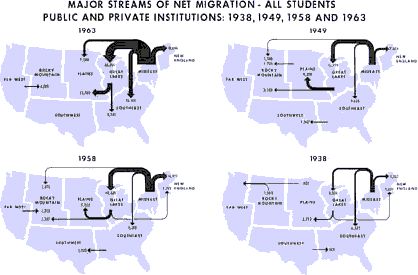
adapted from Migration of College and University Students
in the United States
The size of the arrows indicates the amount of migration. I have heard that midwestern legislators, shown exactly these graphs, were led to invent out-of-state tuition, pitting higher education's prior goal of seeking "foreign" enrollments against the need to deflect some of the costs their universities incurred educating students from the Middle Atlantic and New England states. I'm also told this led, in turn, to the development of the Pennsylvania and New York State University systems. Rank-Size Rule When cities are rank-ordered from largest to smallest, the "rank-size rule" says that the r-th largest will be 1/r-th the size of the largest city, i.e., rank-times-size is a constant equal to the size of the largest city. The equation is where R is rank and sr is the size of the r-th ranked city. It was first noted by Auerbach[17], for the 94 largest cities in the German census of 1910. Lotka[18] reformulated the rule, with an exponent for R which need not be unity. Zipf[19] popularized it, providing numerous empirical examples. The rule has been found to apply to cities in the United States, Canada, most European nations, Japan, Malaya, India and even to cities of the world taken as a whole.[20] There have been a number of attempts to derive it theoretically.[21] Fig. 9-3a shows the distribution of city sizes in the United States, 1980, for the 173 cities larger than 100,000.[22]
Fig. 9-3b shows rank-times-size as Auerbach did it originally. The rank- size rule seems to hold for cities beyond rank 50, but the "constant" descends fairly steadily from rank 50 down to rank 1. It might be argued that rule is still good, but that largest cities are prevented from growing by the suburbs which ring them, producing a sort of "pathology" in the city-size distribution. That is beyond the scope of this study.
Fig. 9-3c shows the rank-size distribution as Zipf and others typically present it. Here the rule does appear to fit a downward sloping straight line.
Human interaction takes time, whatever its content. As the size s of a group increases, the number of possible interactions increases by a factor of s(s-1). The quantity s(s-1) tends to equal s2 as s becomes large. If a society had only this time factor to contend with, the time-minimization solution would be a set of N uniformly small cities, each sized s, with the total population equal to Ns. But, as usual, there are compensatory factors. Large groups may increase the interaction time within groups, but they provide time savings as well. They provide large, diversified markets, for specialized labor and commodities, and there are often economies of agglomeration resulting from the clustering of related activities. If this were the only factor to consider, the time-minimizing solution would be one large city containing the entire population. There should be an optimum between these contradictory time-minimizing arrangements. One possibility would be a fairly small number of fairly large groups, but this would deny society the benefit of both extremes. Another solution, one which permits a much greater range of sizes, would be to make the probability of finding a group of a given size inversely proportional to the interaction time where c is the constant of proportionality. A graph of this equation is shown in Fig. 9-3d. City size, which mathematically could range from 1 to infinity, takes empirical values from the smallest city sn to the largest s1, with cities of varying rank sr in between.
The area under the curve in Fig. 9-6, over the entire range from sn to infinity can be obtained by integration[23] of Eq. 13 between the limits sn to infinity Since the total probability over the entire range must equal 1.0, it follows that c = sn. Substituting this value, we can determine the probability of finding a group equal to or less than sr The probability of finding a group greater than or equal to sr is therefore This probability, multiplied by the number of groups N, gives the rank[24] Multiplying this equation by sr Since N and sn are given, it follows that The rank-size rule is derivable from the assumption of time-minimization. We have assumed that the advantages and disadvantage of small and large towns "balanced out", that the time-savings due to decreasing interaction were equally balanced by the time-savings realized through increasing interaction. If we let d/i represent the advantage of decreasing interaction over that of increasing it, we may begin the derivation with this version of Eq. 13 and obtain the result
This handles the modification introduced by Lotka,[25] with an exponent for R which need not be unity. The result is a logged size-density line with slope i/d (= 1 in the special case i=d). Square-Cube Law A rather different empirical regularity was reported by Mason Haire[26] dealing with what he called the "square-cube law" of formal organizations. Haire's own illustration of the relationship is shown in Fig. 9-7[27].
Haire examined longitudinal data for four firms. He divided the employees of these firms into "external employees", those who interact with others outside the firm, and "internal employees", those who interact only with others inside the firm. He found that the cube-root of the number of internal employees was directly proportional to the square-root of the number of external employees, which we can express with the equation: where a is the intercept and b is the slope. Haire's explanation was based on an analogy with physical objects. Increasing the length of the side of a cube by a factor of 10 increases the surface area by a factor of 10-squared (100) and the volume by 10- cubed (1000). He cities D'Arcy Thompson[28] who applied such dimensional analysis to various biological phenomena. Without entering the debate over the empirical adequacy of Haire's "law", [29] which seems to have been mostly a debate over curve-fitting, we supply a theoretical derivation from the assumption of time-minimization. I assume the existence of a firm, separable from its surroundings, with measurements called E and I, presumably designating external and internal employees as described by Haire. We assume that the benefits which accrue to the firm come in from the environment through the effort of its external employees, so that they in effect support themselves (as well as the firm). The internal employees must, in a sense, ride on the back of the external employees, their "support cost" increasing in proportion to their number relative to the number of external employees: If there were no internal employees, the external employees would have to coordinate their activity themselves. This would involve a time-cost proportional to their interaction time, E(E-1), which, as E becomes large, approaches E2. The "coordination cost" goes down with increases in the number of internal employees, so we have The total time expenditure involving the reciprocal relations of these two groups of employees is thus Assuming that E is given (by organizational-environmental conditions) how large should I be to minimize the total time expenditure? Differentiating T with respect to I, we obtain
where b is a constant of proportionality. Adding a minimum amount of internal organization, a startup cost, we get the equation we set out to derive. Conclusion We have extended the scope of time-minimization theory in this chapter, beyond the original size-density relation which stimulated its development. [30] We now have six independent empirical generalizations derived from the same initial assumption:
These findings — individually, but especially taken as a whole — strengthen the argument for time-minimization theory. As in the last chapter, I emphasize that none of this is intended to suggest conscious or purposeful time-minimizing. It is hard to imagine deliberate planning behind any of these relations (except possibly the one from formal organization, and even there it is hard to imagine conscious creation of such a law).
NOTES: [1] This brief summary is taken from Alexander Hellemans and Bryan Bunch, The Timetables of Science, New York: Simon and Schuster, 1988. [2] especially so when compared with the humoral (imbalances) and miasmal (bad air) theories which had held the metaphysical stage since ancient times. [3] John Q. Stewart and William Warntz, "Physics of Population Distribution", Journal of Regional Science, 1:90-123, 1958. [4] William F. Ogburn and Otis Dudley Duncan, "City Size as a Sociological Variable", Pp. 58-76 in Ernest W. Burgess and Donald Bogue (editors), Contributions to Urban Sociology, Chicago: University Press, 1964. [5] John Q. Stewart, "Potential of Population and its Application in Marketing", Pp. 19-40 in R. Cox and W. Anderson (editors), Theory in marketing, Homewood, IL: Irwin, 1950; and Chauncey D. Harris, "The Market as a Factor in the Localization of Industry in the United States", Annals of the Association of American Geographers, 44:315:348, 1954. [6] G. Edward Stephan and Lucky M. Tedrow, "A Theory of Time-Minimization: the Relationship between Urban Area and Population", Pacific Sociological Review, 20:105-12, 1976. [7] R. H. Best, A. R. Jones and A. W. Rogers, "The density-Size Rule", Urban Studies, 11:201-8, 1975. [8] Ernest W. Burgess, "The Determinants of Gradients in the Growth of the City", Publications of the American Sociological Society, 21:178-84, 1927. William Peterson, Population (3rd edition), New York: Macmillan, 1975: p 476 notes: "[Burgess] first offered his theory of urban zones in a paper read before the American Sociological Society in 1923 and developed it into a mature statement by 1929", but neither paper is cited. [9] Here is one example (Peterson, Op. Cit., p 477): For a full generation or more, the density gradient dominated both theory and research in urban sociology, particularly at Chicago. Monographs were written on the spatial distribution of crime and delinquency, family patterns, mental disorders, and other social characteristics; and all seemed to validate the theory. Then a decade or two after its initial formulation, the hypothesis of concentric circular zones was subjected to a good deal of criticism, both theoretically and empirically based. Although the studies of some cities in addition to Chicago seemed to confirm the hypothesis (St. Louis, Rochester), others apparently had more complex and altogether different spatial patterns (New Haven, Boston, Pittsburgh, New York, Flint). According to even a sympathetic critic [James Quinn], 'The hypothesis of concentric zones as formulated by Burgess needs to be seriously modified if, indeed, it can be defended at all.[10] Homer Hoyt, The Structure and Growth of Residential Neighborhoods in American Cities. Washington. 1939. "Structure of American Cities in the Post-War Era", American Journal of Sociology, 48:475-492, 1943. [11] Chauncey. D. Harris and E. L. Ullman, "The Nature of Cities", Annals of the American Academy of Political and Social Science, 242:12, 1945. [12] The earliest explicit formulation was by Henry C. Carey, Principles of Social Science, Philadelphia: Lippincott, 1858. It was given formal structure by John Q. Stewart, "An Inverse Distance Variation for Certain Social Influences", Science, 93:89-90, 1941 and extensive empirical support by George K. Zipf, Human Behavior and the Principle of Least Effort, Cambridge: Addison-Wesley, 1949. [13] Gerald A. P. Carrothers, "An Historical Review of the Gravity and Potential Concepts of Human Interaction", Journal of the American Institute of Planners, 22:94-102, 1956. Gunnar Olsson, Distance and Human Interaction: A Review and Bibliography, Philadelphia: Regional Science Institute, 1965. [14] Brian J. L. Berry, Geography of Market Centers and Retail Distribution, Englewood Cliffs: Prentice-Hall, 1967 [15] see an example in William R. Catton, Jr., "From Animistic to Naturalistic Sociology, New York: McGraw-Hill, 1966. [16] E. G. Ravenstein, "The Laws of Migration", Journal of the Royal Statistical Society, 48(Part 2):167-277, 1885 and "The Laws of Migration", Journal of the Royal Statistical Society, 52: 241-301, 1889. The effect of improved technology was the sixth of Ravenstein's seven "laws". [17] Felix Auerbach, "Das Gesetz der Bevolkerungskonzentration", Petermanns Mitteilungen, 59:74-6, 1913. [18] Alfred J. Lotka, Elements of Mathematical Biology, New York: Dover, (1924)1956. [19] Zipf, Op. Cit. [20] Charles S. Gossman, The Rank-Size Rule and Mathematical Models for the Size Distribution of American Cities, M.A. Thesis, Department of Sociology, University Washington, 1966. [21] H. W. Richardson, "Theory of the Distribution of City Sizes: Review and Prospect", Regional Studies, 7:239-51, 1973. [22] U.S. Bureau of the Census, Statistical Abstract of the United States: 1986, :Table 19, Washington, D.C., 1985 [23] integration: This is in the methodological appendix.
[24] The rank of the smallest city, size
s [25] Op. Cit. Note that d/i may be regarded as the ratio of what Zipf (Op. Cit.) called the "force of diversification" and the "force of unification". [26] Mason Haire, "Biological Models and Empirical Histories of the Growth of Organizations", in Mason Haire (editor), Modern Organization Theory, New York: Wiley, 1959. [27] adapted from Haire, Op. Cit., p 286 ("Company B"). [28] D'Arcy Thompson, Growth and Form, Cambridge: The University Press, 1952. [29] see D. H. Carlisle, "A Biological Model as an Explanation for the Growth of School Organizations", Journal of Educational Research, 62:313-4; J. Draper and G. Strother, "Testing a Model of Organizational Growth", Human Organization, 22:180-94; S. Levy and G. Donhowe, "Explanations of a Biological Model of Industrial Organization", Journal of Business, 35:335-42; and W. H. McWhinney, "On the Geometry of Organizations", Administrative Science Quarterly, 10:345-63. [30] Three derivations (urban populations, gravity model, and rank-size) are in G. Edward Stephan, "Derivation of some Social-Demographic Regularities from the Theory of Time-Minimization", Social Forces, 53:812-23, 1979. Derivation of the square-cube law is in G. Edward Stephan, "Deriving the Square-Cube Law of Formal Organizations from the Theory of Time-Minimization", Social Forces, 61:847-54, 1983. | ||||||||||||||||||||||||||||||||||||||||||||||||||||||||||||||||||||||||||||||||||||||||||||||||||||||||||||||||||||||||||||||||||||||||||||||||||