Chapter 14
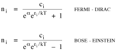
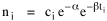
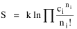
Time, Probability and ThermodynamicsA human being is part of a whole, called by us the Universe, a part limited in time and space. He experiences himself, his thoughts and feelings, as something separated from the rest--a kind of optical delusion of his consciousness. This delusion is a kind of prison for us, restricting us to our personal desires and to affection for a few persons nearest us. Our task must be to free ourselves from this prison by widening our circles of compassion to embrace all living creatures and the whole of nature in its beauty.NOTE: The mathematics in this chapter may be difficult for some readers. The chapter is not essential to the general theme of the book. It is tangential. So feel free to skip it if it doesn't interest you. In 1977 I gave a talk about my research on size-density to an audience primarily composed of members of the science departments at Western Washington University. After the talk the Chairman of the Physics Department, Louis Barrett, walked with me in the direction of our offices. My remarks about the forces shaping population distributions had prompted him to think of analogies with the distributions of physical particles. By the time we reached his office we were joking about whether humans were "fermions" or "bosons" (explanation follows). Before I left, he had me taking the joke seriously and, when I said I wanted to pursue it further, he gave me a textbook[1] to read. All physical particles are governed by one or the other of two statistical distributions, the Fermi-Dirac distribution or the Bose-Einstein. Fermions, which include protons, neutrons and electrons, obey the "exclusion principle": no two can occupy the same quantum state. Bosons, which include photons, alpha particles and helium atoms, do not obey the exclusion principle. The distribution formulas are
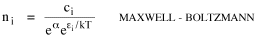
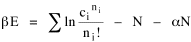
where ni is the number of particles whose energy is εi and ci is the number of states that have the same energy εi. Under the exclusion principle the "occupation index", ni/ci, cannot be greater than 1. At low temperatures virtually all the lower energy states are filled, and the two distributions differ from one another. But at higher temperatures the occupation index is sufficiently small at all energies for the effect of the exclusion principle to be unimportant. They each become similar to a distribution governing particles which, like gas molecules, are sufficiently widely separated to be distinguishable from one another:
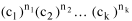
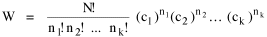
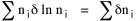
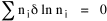
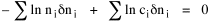
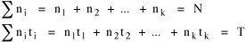
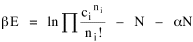
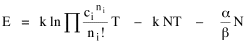
I began to think about energy in physical systems as somehow equivalent to time for living systems. Both can be used to do work, both can be spent, wasted, manifested in a variety of ways. In the textbook Lou gave me is the sentence: "A system of particles is stable when its total energy is a minimum."[2] Perhaps that was the trigger; I don't remember. At any rate, I substituted time for energy in the Maxwell-Boltzmann distribution (humans can be distinguished from one another, by other humans at least), skipping any other direct physical analogies in the textbook derivation. The beauty of the derivation, to me, is the bare minimum of assumptions. Maxwell-Boltzmann Distribution We begin by specifying a random variable t, the time which various individuals expend on some activity. We wish to know the most probable distribution of the individuals across increasing expenditures of time: n1,n2,...,nk at levels t1,t2,...,tk. The total number of individuals N is Σni, and the total time expended by them T is Σtini. We assume that the most probable distribution will be the one which can occur in the greatest number of ways. Pursuant to this we must determine the number of ways in which a given distribution can occur. If there are ci cells in a sample space having the value ti then the number of ways in which one individual could expend the time ti is ci. The number of ways in which two individuals could expend the time ti is (ci)2, and the total number of ways that ni individuals could expend the time ti is (ci)ni. Thus, the number of ways in which all N individuals can be distributed among the various levels of T is the product There are N! permutations among N individuals. But the ni! permutations within the i-th level will not affect the overall distribution. Since there are n1!n2! ... nk! of these irrelevant permutations, the number of relevant ones is The number of ways in which N individuals can be distributed among the possible levels of T is therefore The logarithmic transformation of which is By Stirling's formula, when n is very large so and, since Σ ni = N, We want to find the condition under which W is a maximum, but we have an expression for ln W rather than W; this is not a problem since (ln W)max = ln Wmax. If W = Wmax then small changes δni in any of the ni's will not alter the value of W, so Since N ln N is a constant, it follows that Since so that and since, with N fixed, Σ δni = 0, it follows that Eq. 4 thus becomes While Eq. 5 must be fulfilled by the most probable distribution, it does not fully specify that distribution. There are two constraints to take into account, namely, that the number of individuals and the total amount of time available to them are given: It follows that the variations δni in any of the ni's cannot be independent of one another but must obey the relationships:
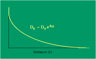
To incorporate these two conditions on the δni's in Eq. 5 we make use of Lagrange's method of undetermined multipliers. We multiply Eq. 6 by -α and Eq. 7 by -β, where α and β are independent of the ni's, and add these expression to Eq. 5. We obtain For each of the equations which enter into the sum in Eq. 8, the variation δni is effectively an independent variable. For Eq. 8 to hold, then the quantity in parentheses must be 0 for each value of i. As a result from which we obtain With time as a continuous variable and n(t) dt as the number of individuals between t and t+dt, Eq. 10 becomes I wanted to see if this distribution function could be applied to some sociological phenomena. In Chapter 9 I suggested that time minimization might lead to the traditional concentric zone model for cities. In the next section I review some work in this area[3] involving more precise statements about population distribution as a function of distance from the center of a city. Following this I address the same problem using Eq. 11 as a starting point. Distribution of Urban Population Using small-area, census-tract type units for cities in Europe, North America and Australia, Clark[4] determined that urban populations decline exponentially from the center, describing a curve such as that in Figure 14-1.
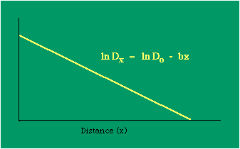
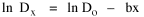
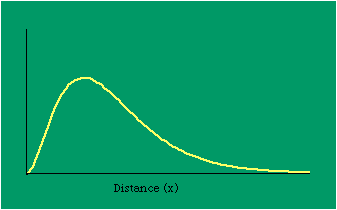
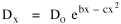
Dx, the density at distance x, declines at the rate b (called the "density gradient") from its value at zero distance Do (called the "central density"). The equation is ordinarily transformed from to permitting estimation of b from linear regression of ln Dx on x. This results in a direct estimate of b (the slope) and an indirect estimate of Do (the antilog of the intercept). Clark computed values for b and Do for such cities as London, Paris, Berlin, New York, Chicago and Brisbane, through the nineteenth and the first half of the twentieth centuries. He noted a tendency for the slope to be less steep over time, and also a tendency for the central density to rise for a while then drop again. Both tendencies were viewed as typical of urban expansion. With these slight variations, he concluded that the negative exponential distribution appeared to hold "for all times and places studied, from 1801 to the present day, and from Los Angeles to Budapest".[5] Later empirical work, summarized by Berry, et al. [6] showed very widespread support for Clark's equation, though they suggest some variation for non-western cities (slopes tending to be constant over time, central density steadily rising). They concluded with an echo of Clark's own assessment: "Regardless of time or place, the expression ... provides a statistically significant fit to the distribution of population densities within cities".[7] One weakness with Clark's curve, recognized from the very beginning, is that the central density, however necessary in order to fix the height of the curve, is fictional: It is found only by extrapolating the regression line inward from the outer residential areas. Theoretically, Clark's curve suggests that the density at dead center should be infinity; that is, the distance x can be made so small that the density created by a single person would approach infinity. If one person occupied one square foot at dead center, the density there would be the number of square feet in a square mile, 27,878,400. Actual residential densities, of course, are never this high. As Burgess' model (Fig. 9-2) suggests, actual central densities tend rather to be quite low, much lower than any extrapolated value. As in Fig. 14-2, the curve usually rises from a very low central value, peaks some distance from the center, and only then begins the exponential decline described by Clark's curve.
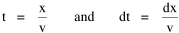
The problem with the concentric zone curve in Fig. 14-2 is that it is only qualitative. It lacks the precision of an equation which could be tested using real data. Newling[8] suggested a modification of Clark's formula
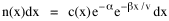
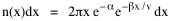
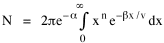
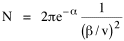
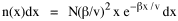
so that it could rise before beginning its decline, but this really is an exercise in curve fitting: if you keep adding enough parameters you can fit anything to any equation. What we want is a curve which can be fit to real-world data and which also has theoretical rationale behind it. Maxwell-Boltzmann Urban Populations The general theoretical result, Eq. 11, can be applied to the problem of determining the distribution of population as a function of distance from the center of a city. The obvious link between distance x and time t is the velocity from which it follows that Making these substitutions in Eq. 11 we have The number of cells in the sample space, at the distance x, should be a function of the circumference at that distance With this substitution, Eq. 14 becomes We can evaluate the constant e -α. Integrating Eq. 16
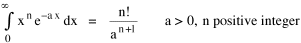
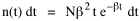
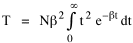
Since the definite integral [9] Eq. 17 becomes, with a = β/v and n = 1 so Substituting this in Eq. 16, To evaluate β, we compute the time T. From Eq. 13 we obtain so we can re-write Eq. 20 as Total time T is Substituting from Eq. 21, By the definite integral used to derive Eq. 18, this becomes
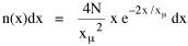
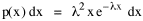
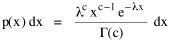
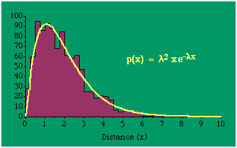
Since T/N is the mean time, and since x = v/t, it follows that the mean distance xμ = vT/N, so Substituting this in Eq. 20, Dividing Eq. 26 by N produces the probability distribution where λ = 2/xμ. This is the gamma distribution[10] with c = 2. The mode of a gamma distribution is (c-1)/λ, so the mode of Eq. 27 is 1/λ and, therefore, λ = 1/mode. The gamma distribution parameters λ and c can be estimated from the mean and variance of x, by the method of matching moments, with
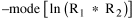
Random numbers fitting this distribution may be generated from where R1 and R 2 are random numbers between zero and one. Fig. 14-3 shows the distribution of 1,000 random distances created using Eq. 30 and the curve generated using Eqs. 28 and 29, mode = 1.94, s 2 = 1.75, implying λ = 1; c = 2.25.
All that is needed to extend this technique to other distributions is to define the two time-components in Eq. 11 with reference to some specific time-expenditure. In the example here, time was related to distance, and the number of cells having the same time was given by the circumference. In a sense it looks as though Clark's distribution results from failing to think in two dimenisional (area) terms: you obtain his equation by moving linearly outward from the center, ignoring circumference, so that c(t) = 1. Each time-distance can be occupied by only one individual (the exclusion principle?) If time expenditure involved an initial startup cost and then decreased in importance over long distances, you might be able to set t = bx -cx 2, i.e., Newling's distribution. Many kinds of distributions[11] can be generated through similar manipulations of the two components. With c(t) = 1 and t = ln x (logarithmic relations are suggested in many areas of human response, i.e., the Weber-Fechner law or the law of proportionate effect), you get p(x) ∝ x-β, commonly known as the Pareto distribution. When β = 1 this is Zipf's law (the rank-size rule). Mandlebrot has derived a distribution of word frequencies which assumes the determining factor to be the time it takes to encode-decode words, p(x) ∝ (m + x)-β. This is the Pareto-type assumption with a minimum or startup time, m (the time it takes to recognize a word, prior to decoding it?): t = ln (m + x). Thermodynamics So far in this chapter I have resisted the temptation to draw direct analogies between Physics and Sociology. Analogy can be an intellectual trap. We call the interactance hypothesis the "gravity model" because it looks like the formula for gravity, but we know that there are differences between migration and gravitational attraction. People may or may not share a time level (be subject to the exclusion principle), but that doesn't literally make them bosons or fermions; we don't investigate their wave functions or spin properties. The only analogy employed in obtaining Eq. 11 was that between energy and time. Beyond that we only assumed a fixed number of individuals with the given amount of time, and that the distribution which could occur in the greatest number of ways was the most probable, assumptions which need not be limited to physical particles. At this point I am going to develop an analogy, or at least the structure for it, solely because I find it intriguing. It should have application in Sociology; at least I can't see any reason for restricting it to physical particles. But I don't know how to make the application. For convenience, and because I can't suggest any immediate application of the energy-time equivalence, I'm going to develop this derivation using e, the symbol for energy. Starting with Eq. 9 I rearrange the terms and multiply both sides by ni Then take the sum of both sides and add Σ ni = N = 0 Combining terms and applying Stirling's formula Continuing to combine terms Since Σ ln x = ln Π x In Physics the constant β is defined where T is temperature and k is "Boltzmann's contant" (1.380 x 10⁻²³ J/molecule-degree). Dividing Eq. 36 by β therefore yields With the following identities, defined in Physics, we arrive at the "fundamental equation"[12] of thermodynamics. It says that the total energy in a system is entropy-times-temperature minus pressure-times-volume plus the chemical potential of the N particles in the system.
And what is entropy — unpredictability? is that what we call freedom? What is the social equivalent of the product entropy-times-temperature? Freedom of movement? What do pressure and volume suggest, if anything? Could the raw product kNT be given some sociological meaning? Do humans have something like chemical potential, some sort of (bonding) potential? Maybe the last two terms in Eq. 36 could be combined into something with a meaning specific to Sociology. Combining them into -N(1 + α), with N as a population — what would be the sociological significance of the factor -(1 + α)/β? Could the value for β computed above in the case of urban population distributions (β = 2v/xμ) have any application? I don't know. NOTES: [1] Arthur Beiser, Concepts of Modern Physics, 2nd ed., New York: McGraw-Hill, 1973. [2] ibid., 213. [3] begun with an undergraduate, Monte Jarvis, in 1988. He went to graduate school (University of Pennsylvania); we never completed it. [4] Colin Clark, "Urban population densities", Journal of the Royal Statistical Society, Series A, 114:490-96, 1951 [5] ibid., 475. [6] Brian J. L. Berry, James W. Simmons and Robert J. Tennant, Urban Population Densities: Structure and Change", Geographical Review, 53:389-405, 1963. [7] ibid., 403. [8] Bruce Newling, "The Spatial Variation of Urban Population Densities", Geographical Review, 59:242-52., 1969. [9] Samuel M. Selby, ed, Standard Mathematical Tables, 19th ed., integral 661, p 449, Cleveland, OH: Chemical Rubber Company., 1971. [10] for this and other properties of the gamma distribution, see N. A. J. Hastings and J. B. Peacock, Statistical Distributions, 54-5, New York: John Wiley & Sons, 1975. [11] for these and many other distributions, see Hastings and Peacock, Op. Cit.(the Pareto is p. 120). also see B. Mandlebrot, "Jeux de Communication", Publ. de l'Inst. de Statistique de l'Univ. de Paris, summarized in Leon Brillouin, Science and Information Theory, 2nd ed., New York: Academic Press, 1953. [12] Edward A. Desloge, Thermal Physics, p 156, New York: Holt, Rinehart and Winston, 1968 |