CHAPTER 13
Erosion of the Size-Density RelationIn Chapter 12 it appeared that slopes more negative than -2/3 were the result of including cities in the analysis. In this chapter we examine the reverse condition: slopes less negative than -2/3, slopes tending toward zero (which is to say tending toward no slope or relation at all).At the conclusion of the article in which we presented the results of the last chapter, we added the findings shown in the next table, comparing our latest slopes with the earliest ones for which we could obtain data.[1] We were attempting to see if other countries might have experienced the kind of "erosion" of a -2/3 size-density slope which we saw earlier in England (Chapter 7).
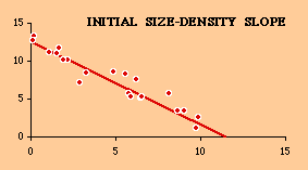
It is evident that in every case the earlier slope is closer to -2/3. The earlier slopes for Italy, Netherlands, Portugal and Spain, in fact, conform to the hypothesis by the p > .05 criterion. Even in the case of France, the p-value improved from .00000005 to .00008, suggesting that, if we had still earlier data, départements which were intended to be uniformly small still might have shown some conformity to the size-density law. We developed a tentative explanation for the tendency of slopes to erode toward zero. If boundaries remain fixed while the population experiences redistribution, then any relation which once existed will, obviously erode; you can't change the independent variable while holding the dependent variable constant and expect the original relation to persist. More particularly, suppose we have a set of territorial divisions which do fit the size-density law. Now fix the boundaries of the territorial divisions once and for all. This could happen through historical inertia (e.g., England) or technological change (e.g., the automobile and U.S. counties). Under normal processes of population growth high-density places will tend to become even more dense. This is the law of proportionate effect: nothing succeeds like success, the rich get richer, big population centers draw more people than small ones (gravity model). Ordinarily such growth would lead to further subdivision (down to some technologically/economically minimal size), but here no further subdivision occurs. The result is erosion of the slope. This is easily simulated An initial group of 20 data points, scattered around a regression line (exact-fit points were computed, then a random number was added or subtracted from the vertical coordinate).
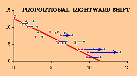
Next we move data points to the right. The arrow points have the same vertical coordinates as the original data points (no change in area), but the horizontal coordinates have been increased. The amount of increase is proportional to the original value, plus a positive or negative random number. The new data points resulting from the rightward moves are shown in green.
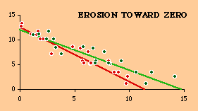
Finally, we compute a new regression line for the generated points. The slope has eroded has clearly eroded toward zero.
As originally put forward, the erosion hypothesis was only suggested, along with the data in Table 13-1 confirming that earlier slopes tended to be more negative. In 1982, with the help of my wife Karen,[2] I conducted a direct test of the erosion hypothesis. The question was: Does the slope become less negative as population becomes more concentrated? We needed area and population data for stable sets of territorial divisions over significant periods of time. Ideally, stability would mean no change whatever in the boundaries of divisions throughout the period of study. We found such data[3] for Austria (9 Bundesländer: 1910-1961)We also included studies[4] of three nations where the number of changes in territorial divisions was small relative to the number of divisions Italy (14 Regioni: 1861-1911; 15: 1921-1951)We computed size-density slopes for each of the years indicated in the accompanying table: .
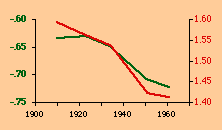
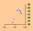
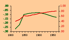
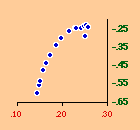
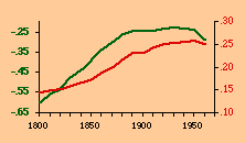
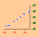
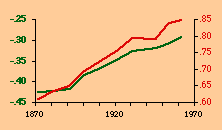
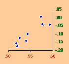
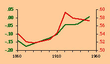
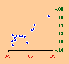
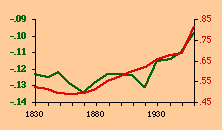
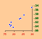
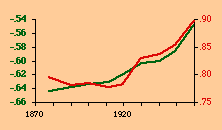
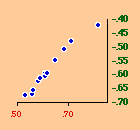
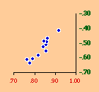
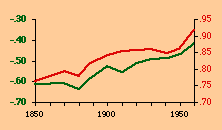
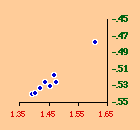
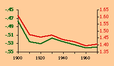
There are a variety of concentration measures which might have been computed[5] We chose the standard deviation of log D (referred to in the table as S.D.). It seems to have escaped the attention of most authors[6] that any measure of concentration can in the end be shown to be based upon this mundane statistic. A standard deviation of zero indicates no concentration (even densities), with increasing values indicating increasing concentration. The standard deviation suffers from the fact that we cannot appropriately compare it across sets with different numbers of divisions. But it is perfectly suitable for our purposes. Figs. 13-1 through 13-10 show historical values for slopes and standard deviations. To the left of each historical graphs is a scatter diagram showing the relation between the two. The size-density slopes are shown in green; the standard deviations (concentration measures) are shown in red. It will be obvious that the two are strongly related (increasing concentration leading to erosion of the slope). A following statistical table summarizes the results of our analysis.
The first is a test of significance, against the null hypothesis, for the linear correlation coefficient[7]. In some cases, e.g. Belgium, the relation is clearly not linear. Nothing in our erosion hypothesis suggests that it should be; we only expect a monotonic increase of the one with the other, i.e., an ordinal relation. For this reason two additional test statistics are provided, Spearman's rho, and Kendall's tau. Hays and Winkler[8] review the advantages and disadvantages of each as an alternative to r-square, concluding ...each index supplies information of importance about the general monotone relation that may exist between variables, quite irrespective of the true value of the correlation coefficient.... For moderately large samples, ... tau seems to provide a better test of the hypothesis of no association....Austria, Fig. 13-1, interestingly, shows support for the hypothesis but in the reverse historical order expected. Over time the population has become less concentrated, and the size-density slope has become steadily more negative, even passing the theoretically expected - 2/3 value. A similar pattern shows up in the United States, Fig. 13-10: here the decreasing concentration reflects increased settlement in large states such as California. This may be more a problem of the level of measurement of area and density, i.e., the state vs. the county. The historical charts for the other nations show remarkable conformity to the notion that size-density tends to erode toward zero over time. The chart for France, incidentally, projected back another century, would produce a slope slightly more negative than -1/2, supporting our earlier conjecture that — even when a deliberate effort is made to produce uniformly size divisions — the size-density relation tends to surface.
NOTES: [1] B. R. Mitchell, European Historical Statistics, New York: Columbia University, 1975. [2] The study was published as G. Edward Stephan and Karen H. Stephan, "Population Redistribution and changes in the Size- Density Slope", Demography, 21:35:40, 1984 [3] The data for Austria, Belgium, France, Netherlands and Switzerland came from Mitchell, Op. Cit.; England and Wales data were from B. R. Mitchell and H. C. Jones, Second Abstract of British Historical Statistics, Cambridge: Cambridge University Press, 1971; United States data was from the census. [4] Mitchell, Op. Cit. [5] I have reviewed a number of these measures and shown that each can be given a probability interpretation: G. Edward Stephan, "Measures of Population Distribution: A Probability Interpretation", Western Sociological Review, 7:3-10, 1976. [6] except notably Maurice G. Kendall and Alan Stuart, The Advanced Theory of Statistics (3 vols.; 2nd ed.), New York: Hafner, 1963. [7] (this will be in the methodological appendix) [8] William L. Hays and Robert L. Winkler, Statistics: Probability, Inference and Decision, 849, New York: Holt, Rinehart and Winston, Inc., 1971. |