Regression and Correlation

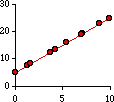
Regression and correlation. The red dots in this diagram form an exact pattern, a straight line which happens to have the formula Y = 5 + 2 (X)

where 5 is the intercept (the value of Y at X=0) and 2 is the slope (the amount by which Y changes as X increases by one). For any value of X there is a precisely corresponding value of Y. The reverse is also true; that is, given any value of Y you could compute the corresponding X-value: (Y - 5) / 2.

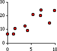
This next figure shows a strong connection between X and Y but not an exact one.

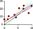
Here large values of X are clearly associated with large values of Y, but the dots don't form a perfect straight line. We could draw one through them. In fact we could draw many different ones through them. Like these:

That's the problem: which line "fits" the dots "best"? There is no absolute or universal answer to that question. It depends what you want the line to do. Often, what we want it do is predict values of Y once we're given values of X -- given an X-value, what do you expect Y to be? We want a line through the dots which refers to the Y-axis.

Let's look at this a little closer. We want a line (formula) which we can use for predicting Y-values. Obviously it will have a formula like Y = a + bX, and our problem is to find numerical values for a and b, given that the observed dots will deviate from whatever line we devise:

It would make sense to choose a and b in such a way that the sum of all the deviations from the line are minimal. The problem here is that we would be summing positive and negative deviations; they would cancel each other out. If we square the deviations each will be a positive value. Let's define "error" then as the sum of the squared deviations, then expand the summed expression and finally distribute the summation:

Our line will be defined by a and b values which minimize this error (since we are minimizing the sum of the squared deviations we are are said to be using "least squares" estimators for the intercept and slope).

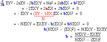
Minimization requires us to find the derivative of this the last expression with respect to both a and b. First, we find the partial derivative with respect to a, set that equal to zero and solve for a:

And now with respect to b (note the substitution of our earlier expression for a, in red):

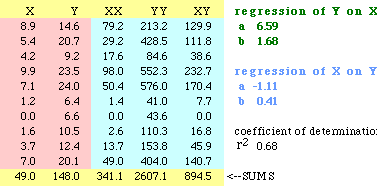
With these equations we can obtain the "least squares regression line" for our data. Here is what the calculation might look like in a spreadsheet:

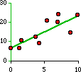
So the regression line for the dots above would be

Y = 6.59 + 1.68 X

As you can see on the spreadsheet, there is nothing to prevent us from calculating the regression line of X on Y (if we wanted to predict X-values from Y-values):

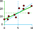
This line, the blue one, isn't exactly the same as the green one. That's because all the dots don't fit on a single line as they did in our first example. In fact, the degree to which the two lines, green and blue, depart from one another can be used as a statement of how well the two variables are related.

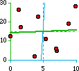
The measure "coefficient of determination" (r-squared, often confused with plain r, the "correlation coefficient") is the product of the two slopes, b from Y-on-X and b from X-on-Y. It varies from 0 to 1 and describes the proportion of the variance in Y which is explained by the linear model: Y = a + bX. Here are three scatter diagrams, two we've already seen plus a third one:

certainty
mathematical function
r-sq = 1.00
Y = 5 + 2X
X = -2.5 + .5Y
order
strong correlation
r-sq = 0.68
Y = 6.59 + 1.68X
X = -1.11 + 0.41Y
chaos
almost no relation
r-sq = 0.00
Y = 14.17 + 0.31X
X = 4.65 + 0.02Y

If I know nothing about the variable Y except its mean, my best predictor for any to-be-observed value of Y is the mean itself. If there is a relation between Y and some other variable X, then I will be better off using Y = a + bX to predict Y, depending on the strength of the relation. As you can see from the third example, when r-squared is very low you're not much better off with the equation than you were with just the mean of Y: knowing the value of X doesn't tell you much about what to expect of Y.